Equivalent connections represent a special case regarding dominance. Two connections are considered equivalent when they merely differ in the selection of transfer stops, but are the same in terms of departure time and sequence of the time profiles used.
If the connections have path legs without a temporal position (DRT, Sharing, PuT Aux), the definition of equivalence is adjusted slightly: all path legs without a temporal position are then treated as a single time profile. In addition, a coinciding temporal position is given if the first and the last part of the path leg, which is made with a regular public transport line, use the same vehicle journey. In particular, this is equivalent to connections of the type "DRT –> public transport line", which board the same vehicle journey at different stops.
If the dominance of equivalent connections is allowed, the connection with the highest priority (smallest numerical value) dominates all connections with lower priority from a bundle of equivalent connections. If the priorities are the same, you define whether the connection should remain with the earliest or latest possible transfer. The transfer priority can be set at stop areas and between two vehicle journeys (planned connecting journeys). The priorities of the levels are added up. The connection with the highest priority (smallest numerical value) remains as connection. A default priority of 8 applies to stop areas and planned connecting journeys. It is assigned to all elements that are not defined.
If equivalent connections are allowed, a larger amount of nearly identical connections can be created. Please note that the choice model cannot account for the hierarchies within a set of connections. In some cases, using the independence factor allows you to compensate for this fact.
|
Note: Deactivating the independence factor while using equivalent connections can lead to unrealistic results. We therefore strongly recommend that you select the Use independence option when allowing equivalent connections. |
Example
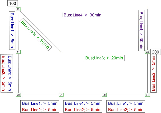
Let us look at the network depicted in Illustration 161.

Illustration 161: Example equivalent connections
When we use lines 1 and 2, the following equivalent connections are created:
| Connection | From-Time profile | To-Time profile | Transfer stop point |
|---|---|---|---|
|
A1 |
Bus, line 1 >, 1 |
Bus, line 2 >, 1 |
11 |
|
A2 |
Bus, line 1 >, 1 |
Bus, line 2 >, 1 |
20 |
|
A3 |
Bus, line 1 >, 1 |
Bus, line 2 >, 1 |
21 |
|
A4 |
Bus, line 1 >, 1 |
Bus, line 2 >, 1 |
30 |
|
A5 |
Bus, line 1 >, 1 |
Bus, line 2 >, 1 |
31 |
If dominance is allowed with equivalent connections, only connection A1 remains available.
Example with independence
| Connection | Path leg(s) |
|---|---|
|
A |
Departure 6:30 AM with line 1 Transfer to line 2 in overlapping area of stop events 11, 20, 21, 30 and 31, TWT = 0 Arrival 7:00 AM |
|
B |
Departure 6:35 AM with line 3 Arrival 7:05 AM |
|
C |
Departure 7:00 AM with line 4 Arrival 7:30 AM |
Without independence factor:
When not using equivalent connections, each of the three connections is assigned a 1/3 share if the impedance parameters are set without a penalty for transfers.
If equivalent connections are allowed, connection A (with transfer at stop event 11) forms the basis for 4 additional options (A2 to A5) that only differ in terms of their transfer point. The set of connections now consists of seven equally good connections, and if the independence factor is not applied, each connection is assigned 1/7 of the demand. This case shows that when the independence factor is not applied, the choice model produces unrealistic results.
With independence factor:
When the independence factor is used in our initial situation, the demand is shifted towards connection C, as the temporal positions of A1 and B are very similar. C is now assigned 47%. The remaining demand is divided between the other two connections.
If equivalent connections are allowed, the share of C hardly changes. However, a large part of the demand shifts from B to A, as A1 to A5 do not only influence each other, but also reduce the independence of B. This case shows that when using the independence factor, you obtain better results. However, it also demonstrates the limits of independence.
|
Independence factor deactivated |
Independence factor activated |
||
|---|---|---|---|
|
Equivalent connections |
Equivalent connections |
||
|
No |
Yes |
No |
Yes |
|
33.3 % |
71.4 % |
26.5 % |
41.8 % |
|
33.3 % |
14.3 % |
26.5 % |
10 % |
|
33.3 % |
14.3 % |
47 % |
48.2 % |

